
Panchapakesan Ganesh, Nikhil Sivadas and Abhijeet Dhakane
Oak Ridge National Laboratory
GITLAB LINK: https://code.ornl.gov/3sd/smc-datachallenge2021/
Ferroelectrics are materials that have spontaneous electric polarization that can be reversed by the application of an external electric field. Existence of a spontaneous polarization implies that the ferroelectric material shows a hysteretic response to the applied field, ideal for use as a memory function, in a ferroelectric random-access memory (FeRAM) device.
Real materials are not pure. They have point and extended defects, buried interfaces as well as domain-walls (i.e., spatial discontinuity in the local polarization vector). In the presence of heterogeneities, in addition to the global order-parameter (i.e., overall spontaneous polarization of the material) there are additional manifestations on the local order-parameter (local polarization), that leads to ‘hidden’ order in the material. As an example, interfaces of different ferroelectric thin-films can show chiral polarization loops, whose formation, stability and motion are not only governed by material properties, but also topological properties. We find that the shape as well as the area of the hysteresis loops are strongly modified by such local order. Further, the dynamics of ferroelectric switching are also significantly modified in the presence of such hidden order in heterogeneous ferroelectrics.
We are specifically interested in discovering such ‘hidden’ order from molecular dynamics simulations and correlate them with the type of heterogeneities present in the simulation. We would like to ascertain how this order influences not just the memory function, but also its ‘dynamics’ under externally applied field. Dynamic control of memory is the basis of ferroelectric-based neuromorphic materials.
We provided the files with local polarization for a length of time for all datasets:
Local polarization of each unit cell (shown in figure below) was calculated using:
where is the volume of the unit cell, ,, are the charges of the Ti, Ba and O atoms obtained using the Electron Equilibration Method (EEM) approach in ReaxFF, and are the positions of the Ti, Ba and O atoms of each unit cell at time t [1].
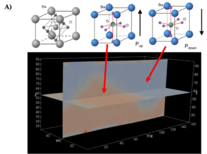
Figure 1: Unit cell schematic of the BaTiO3 (top), for the case with zero-polarization, polarization pointing UP and polarization pointing DOWN, respectively. The bottom figure, generated by PARAVIEW, is a snapshot from the molecular dynamics (i.e. time-series data of local polarization), where the UP regions show up as orange, and DOWN regions as blue. The domain-wall i.e. the interface between the UP/DOWN region should have different dynamics than the rest [2]
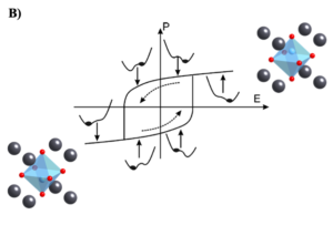
Figure 2: shows the hysteric response of BaTiO3 to an applied electric field. It is not clear how domain wall dynamics differ for different field-values, and control the shape of this loop [2]
The relative atomic motion of Ti-atom as shown in fig. (A) determines the unit cell’s local polarization for a given system. Orange and blue regions are two different symmetric ‘domains’ – domain with Pup and Pdown respectively, with a domain-wall between them. Under an electric-field, say one pointing up, the domain wall move so as to increase the fraction of UP domains. At a particular electric-field, all domains (or almost all) will be converted to a single UP domain. Reversal of the electric-field will result in an increase in the DOWN domain fraction, and the total polarization point up will reduce in magnitude. Interestingly, a plot of the total polarization of the box, when as a function of the electric-field, does not show perfect reversible motion – one sees a so-called hysteresis loop, as shown in fig. (B) – where a change in the total polarization depends on which state it started from, and in which direction is the field applied. This motion (i.e. kinetics and dynamics) of domain walls under fields can be different when defects are present. While in a static snapshot, as shown above, one only sees two domains, different parts of the same domain could show different dynamics or kinetics. We want to identify how many different such ‘dynamical’ states (or domains) exist in our MD simulation when it is in equilibrium? How these dynamical states participate in field-induced switching ? How presence of different defect types change the number of these dynamical states?
Identifying dynamics states, and learning their equation-of-motion, can be performed by combining Koopman’s operator theory of dynamical systems [3] or methods like DMD (Dynamic mode decomposition) method [4], VAE (Variational autoencoders), and TICA (Time-lagged independent component analysis)[5]. This can separate the ‘static’ states from the ‘dynamical’ states from sequential data.
Datasets:
We uploaded two batches of datasets:
Datasets divided into two subsets (a) and (b), each contains different types of defects:
| (a) Equilibrium Dynamics | SET1 (no defects) | VTKFILES, LOCAL_DIPOLE_FILES |
| SET2 (with Ov defect) | VTKFILES, LOCAL_DIPOLE_FILES | |
| SET3 (with Bav defect) | VTKFILES, LOCAL_DIPOLE_FILES | |
| SET4 (with (Ba-O)v defect) | VTKFILES, LOCAL_DIPOLE_FILES | |
| (b) Non-Equilibrium Dynamics | SET1 (no defects) | VTKFILES, LOCAL_DIPOLE_FILES |
| SET2 (with Ov defect) | VTKFILES, LOCAL_DIPOLE_FILES | |
| SET3 (with Bav defect) | VTKFILES, LOCAL_DIPOLE_FILES | |
| SET4 (with (Ba-O)v defect) | VTKFILES, LOCAL_DIPOLE_FILES |
One can visualize the dynamics of the given dataset by using the uploaded VTKFILES using the PARAVIEW software.
LOCAL_DIPOLE_FILES snippet below contains co-ordinate of Ti atoms and local polarization for each snapshot.
# TIMESTEP 250000 0.000000 0.000000 0.000000 162.462759 81.229598 120.800000
2.079 2.043 20.809 0.00505805 -0.00416993 -0.00028926
2.059 2.028 25.018 -0.00045007 -0.00058029 0.00758195
2.085 2.019 29.146 0.00016893 0.00004470 0.00600944
First line, is header contains #TIMESTEP <timestep> <xlow> <ylow> <zlow> <xhigh> <yhigh> <zhigh>
Where unit of timestep is (fs), xlow-xhigh determine the cartesian min/max of the simulation box along the x-direction. Similarly, for y- and z-directions.
Second line onwards, first three columns (column wise) are cartesian co-ordinates of Ti atoms (in Å) while next three columns are the cartesian coordinates of the local polarization vector (in mico-Coulomb/cm2).
The challenge questions are:
Notes:
References:
 Download
 Slack Channel
 Challenge Contact
 Dataset