
Wind flow dynamics at micro-scale are of paramount importance in the wind energy industry. Historically, wind farm designs rely on precise measurements from few meteorological masts over an entire site. However, at microscale, wind flow dynamics can be very sensitive to the terrain irregularities and wind conditions can drastically change from one location to another even over small distances.
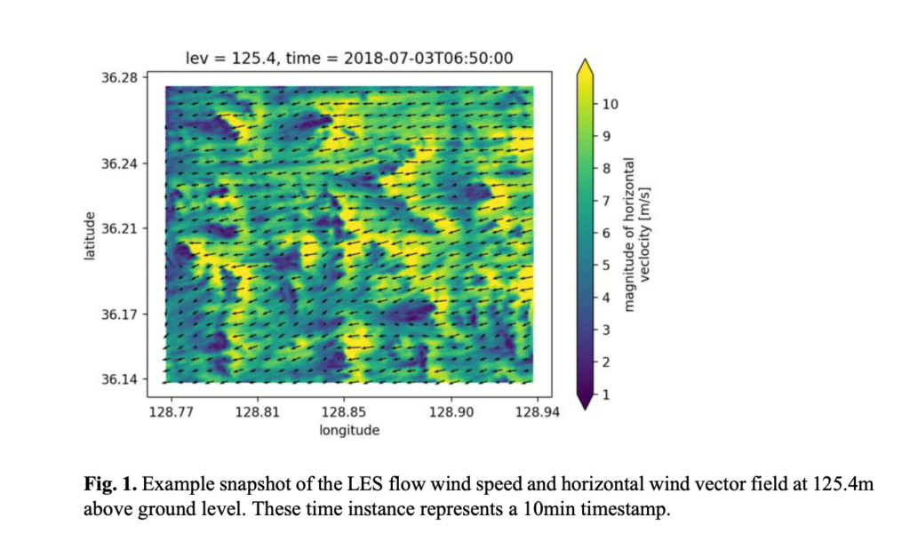
Computational Fluid Dynamics (CFD) is a promising approach for assessing atmospheric flow properties over a domain of interest. In particular, Large Eddy Simulation (LES) is one of the most advanced mathematical models used in CFD for resolving turbulences at a reasonable cost. These simulations use the terrain, the roughness and the global scale forcing (large scale atmospheric flow) to dynamically downscale the wind field at resolution ranging from 10 to 100m. Typical outputs of such calculations are 4D (3D+time) grids of 10min statistics of wind quantities such as the average horizontal wind speed, the standard deviation of the horizontal wind speed or the average horizontal wind direction typically for a year.
ERA5 data is a global weather model at a resolution of ~30km with hourly estimates of atmospheric variables. To summarize, in the present case LES simulations are driven by boundary conditions derived from ERA5 data and then resolve the local wind farm site wind field at much higher resolution in space and time. Hence, quantities from the LES simulation tend to be correlated to ERA5 data. For each site provided, the corre- sponding timeseries from ERA5 is provided.
LES high-resolution datasets are simulations obtained by running a full high-resolution simulation over a period of a year. The typical spatial resolution will be defined and the time resolution is 10min, though the data for this challenge is in an hourly series to make the data download size manageable for the challenge. For the present work, the data will be made available at a single height above ground level. These heights above ground are terrain following slices and are typically centered around the wind turbine hub height. The mesh for the simulation contains therefore 256 x 256 x 1 x 52560 nodes and timesteps.
For each node, timeseries are available for different quantities such as : horizontal wind speed average [m/s], temperature average [K], east-west and north south component of the wind speed [m/s] and absolute height above sea level [m]. The typical size of the LES output for a site is several hundred of GB, however the hourly data or this challenge is only ~7 GB in size.
Please see the Challenge Data Overview below to learn how to obtain the data and a jupyter notebook to get you started.
The data may be obtained from this DOI: https://doi.ccs.ornl.gov/ui/doi/385
The DOI service uses Globus, a non-profit service for secure, reliable data transfer and managment. To obtain the data you must:
The Data DOI contains:
– The dataset for the challenge
– The description of the data
– Python requirements for creating a virtualenv to load the data
– A Quickstart notebook
DOI Folders
├── README.md                               <- This file
│
├── data                                    <- Folder containing the full dataset for the challenge
│   ├── perdigao_era5_2020.nc               <- ERA5 hourly timeseries at single location
│   ├── perdigao_high_res_1H_2020.nc        <- LES hourly grid timeseries at 80m x 80m resolution (8GB)
│   └── perdigao_low_res_1H_2020.nc         <- LES hourly grid timeseries at 160m x 160m resolution (2GB)
|
├── data_samples                            <- Folder containing LES data of the first month of the full dataset (2020-01)
│   ├── perdigao_high_res_1H_2020_01.nc     <- Sample LES hourly grid timeseries at 80m x 80m resolution
│   └── perdigao_low_res_1H_2020_01.nc      <- Sample LES hourly grid timeseries at 160m x 160m resolution
│
├── requirements.txt                        <- Recommended Python libraries for the virtual environment to load the data
|
└── quickstart.ipynb                        <- Quickstart notebook
The data from ERA5 has been downloaded from Copernicus Climate Data Store. data/perdigao_era5_2020.nc corresponds to ERA5 hourly data single levels for the year 2020 (check the documentation here). The data has been extracted at single point (-7.737°E, 39.7°N) since ERA5 spatial resolution is about 30km.
The file format is NetCDF and can be easily opened with xarray (see the python quickstart notebook provided in the DOI for this set).
The data represents hourly timeseries of following quantities (variables are also described in the NetCDF file and Copernicus documentation):
u100: 100 meter above ground level U wind component in m/s.v100: 100 meter above ground level V wind component in m/s.t2m: 2 meter above ground level temperature in K.i10fg: 10 meter above ground level instantaneous wind gust.The full data from LES is available at two different spatial resolutions:
data/perdigao_high_res_1H_2020.nc: 80m x 80m at 1H frequencydata/perdigao_low_res_1H_2020.nc: 160m x 160m at 1H frequencySome samples of the full data is available (NetCDF containing the first month of the full dataset):
perdigao_high_res_1H_2020_01.nc: 80m x 80m at 1H frequencyperdigao_low_res_1H_2020_01.nc: 160m x 160m at 1H frequencyBoth datasets are available at 100m height above ground level i.e. terrain following slices.
Note that the following description of the dataset is also available from the NetCDF files.
Coordinates:
height: Height in meter above ground level (only 100m). This is the height of the terrain following slice for all variables.time: Timestamps at 1H frequency.xf: Horizontal cartesian coordinate in meter of the simulated domain (West to East).yf: Vertical cartesian coordinate in meter of the simulated domain (South to North).Variables:
absolute_height: Height above sea level in meter, note that this variable only depends on (xf, yf) not on time.std: 1H average of standard deviation of horizontal wind speed in m/s originally recorded at 10min frequency.temp: 1H average of temperature in Kelvin.u: 1H average of U component of wind speed (along xf) in m/s.v: 1H average of V component of wind speed (along yf) in m/s.vel: 1H average of horizontal wind speed in m/s.
File formats:
NetCDF files can be opened with xarray python library which is a N-dimensional generalization of pandas.
Besides the quickstart notebook provided with the data, here are some useful links of the documentation to get familiar with xarray:
Have a look at the quickstart notebook and good luck !
1 Exploratory data analysis and visualization
The goal for the first challenge is to get familiarized with the different dataset, compare full grid to single timeseries, quantify differences. As research questions, we propose:
2. Dimensionality reduction of the grid
The goal for the second challenge is to compress the site behavior into a lower dimen- sional space without losing wind flow model properties [1]. As research questions, we propose to answer the following questions:
3. Upscaling from a low-resolution to high-resolution grid
For Large Eddy Simulation, lower resolution simulations are less expensive to generate. Being able to upscale a low-resolution wind grid simulation to accurately match a high- resolution simulation, we can dramatically reduce the simulation cost in terms for com- putational resources and time. In this supervised problem we provide both a low- and high-resolution grid simulations. The objective is to train a supervised model to predict the high-resolution simulation using a low resolution one [2]. These questions should be addressed: